SVD,Eigendecomposition and Mahalanobis (manobala) Distance

Need for Mahalanobis distance

Distance calculated using euclidean geometry provides the absolute value between an origin and the target, yet this quantity lacks on stating how unique/unremarkable a particular point is in a data cluster. Standard deviation of a probability distibution comments on how the variables are spread. Mahalanobis distance is that quantity that tells the measure of a point from the mean in terms of standard deviation. This is particularly required in point clouds because this helps in determining outliers/noise while performing Iterative Closing Point Algorithm.

Formulas to get familiar with

• The Mahalanobis distance is calculated as:

$$d_M (x) = \sqrt{(x - \mu)^\top \Sigma^{-1}(x - \mu)}$$

• Setting $e = x - \mu$ (the deviation from the mean):

$$d_M^2 = e^\top \Sigma^{-1} e = \Vert e \Vert_\Sigma^2$$

• $\Sigma$ is the $d \times d$ covariance matrix

$$\Sigma_{d \times d} = \frac{1}{n - 1} \sum_{i=1}^{n} (\mathbf{x}_i - \bar{\mathbf{x}})(\mathbf{x}_i - \bar{\mathbf{x}})^\top$$

• Let $d=2$, so each observation is a 2D vector $\mathbf{x}_i = \begin{bmatrix}x_{i1}\\ x_{i2}\end{bmatrix}$ and the mean is $\bar{\mathbf{x}} = \begin{bmatrix}\bar{x}_1\\ \bar{x}_2\end{bmatrix}$. The deviation vector for observation $i$

$$\mathbf{x}_i - \bar{\mathbf{x}} = \begin{bmatrix}x_{i1} - \bar{x}_1\\ x_{i2} - \bar{x}_2\end{bmatrix}$$

• The outer product is $(\mathbf{x}_i - \bar{\mathbf{x}})(\mathbf{x}_i - \bar{\mathbf{x}})^\top$. This is a column vector times a row vector — giving a $2\times2$ matrix:

$$(\mathbf{x}_i - \bar{\mathbf{x}})(\mathbf{x}_i - \bar{\mathbf{x}})^\top = \begin{bmatrix}x_{i1}-\bar{x}_1\\ x_{i2}-\bar{x}_2\end{bmatrix}\begin{bmatrix}x_{i1}-\bar{x}_1 & x_{i2}-\bar{x}_2\end{bmatrix}$$ $$= \begin{bmatrix}(x_{i1}-\bar{x}_1)^2 & (x_{i1}-\bar{x}_1)(x_{i2}-\bar{x}_2)\\ (x_{i2}-\bar{x}_2)(x_{i1}-\bar{x}_1) & (x_{i2}-\bar{x}_2)^2\end{bmatrix}$$

note: d is number of features(columns) and n is number of observations (rows)

• Sum over all $n$ observations

$$\sum_{i=1}^{n}(\mathbf{x}_i - \bar{\mathbf{x}})(\mathbf{x}_i - \bar{\mathbf{x}})^\top = \begin{bmatrix}\sum_i(x_{i1}-\bar{x}_1)^2 & \sum_i(x_{i1}-\bar{x}_1)(x_{i2}-\bar{x}_2)\\ \sum_i(x_{i2}-\bar{x}_2)(x_{i1}-\bar{x}_1) & \sum_i(x_{i2}-\bar{x}_2)^2\end{bmatrix}$$

• Divide by $n-1$

$$\Sigma_{2\times2} = \frac{1}{n-1}\begin{bmatrix}\sum_i(x_{i1}-\bar{x}_1)^2 & \sum_i(x_{i1}-\bar{x}_1)(x_{i2}-\bar{x}_2)\\ \sum_i(x_{i2}-\bar{x}_2)(x_{i1}-\bar{x}_1) & \sum_i(x_{i2}-\bar{x}_2)^2\end{bmatrix}$$

Reading each entry

$$\Sigma_{2\times2} = \begin{bmatrix}\text{Var}(x_1) & \text{Cov}(x_1,x_2)\\ \text{Cov}(x_2,x_1) & \text{Var}(x_2)\end{bmatrix}$$

• $(1,1)$: $\frac{1}{n-1}\sum_i(x_{i1}-\bar{x}_1)^2$ — variance of feature 1. Same feature squared with itself.
• $(1,2)$: $\frac{1}{n-1}\sum_i(x_{i1}-\bar{x}_1)(x_{i2}-\bar{x}_2)$ — covariance of feature 1 and 2. Two different features multiplied.
• $(2,1)$: same as $(1,2)$ — always symmetric since multiplication is commutative.
• $(2,2)$: $\frac{1}{n-1}\sum_i(x_{i2}-\bar{x}_2)^2$ — variance of feature 2.

---

Connection to $\frac{1}{n-1}X_c^\top X_c$ (centered data)

The formula $\frac{1}{n-1}\sum_i(\mathbf{x}_i - \bar{\mathbf{x}})(\mathbf{x}_i - \bar{\mathbf{x}})^\top$ and $\frac{1}{n-1}X_c^\top X_c$ are the same thing written two different ways:

• The summation form adds up $n$ outer products one observation at a time
• The matrix form stacks all observations into $X_c$ and does one matrix multiplication

Both produce the identical $2\times2$ covariance matrix — the summation form makes the meaning explicit, the matrix form is compact and fast to compute.

⚠️ Centering requirement: The matrix form only equals the covariance matrix if $X_c$ is mean-centered — each row must be $(\mathbf{x}_i - \bar{\mathbf{x}})^\top$, so every column sums to zero. The summation form has $-\bar{\mathbf{x}}$ built into each term; the matrix form must bake it into $X_c$ itself.

On raw (uncentered) data, $\frac{1}{n-1}X^\top X$ gives the second moment matrix instead:

$$\frac{1}{n-1}X^\top X = \Sigma + \tfrac{n}{n-1}\,\bar{\mathbf{x}}\bar{\mathbf{x}}^\top$$

equal to $\Sigma$ only when $\bar{\mathbf{x}} = \mathbf{0}$.

Centering ≠ normalising. The ladder:

• Raw $X$ → second moment matrix
• Centered $X$ → covariance matrix $\Sigma$ ← what Mahalanobis needs
• Centered + scaled by std dev → correlation matrix $R$ Worked example (1 feature, $n=3$): let $x = [1, 2, 3]$, so $\bar x = 2$.

Centered: $x_c = [-1, 0, 1]$

$$\frac{1}{n-1}x_c^\top x_c = \frac{1}{2}\left[(-1)^2+0^2+1^2\right] = 1$$

This matches $\text{Var}(x) = \frac{1}{n-1}\sum_i(x_i-\bar x)^2 = 1$ exactly. ✓

Raw (uncentered): using $x = [1,2,3]$ directly

$$\frac{1}{n-1}x^\top x = \frac{1}{2}\left[1^2+2^2+3^2\right] = \frac{14}{2} = 7$$

7 is not the variance — it’s inflated by the mean not being zero. This is exactly $\Sigma + \frac{n}{n-1}\bar x^2 = 1 + \frac{3}{2}(2)^2 = 1 + 6 = 7$. ✓

Skipping the centering step silently swaps “spread around the mean” for “spread around zero” — the two only agree when $\bar x = 0$.

Note: The query point $x$ in $d_M(x)$ never needs pre-centering — the $(x - \mu)$ inside the formula centers it explicitly. Centering only matters for how $\Sigma$ is computed from the data matrix.

What is covariance, variance and standard deviation? and Ohh my Gaussian Curve

• $\sigma^2$ is variance — the average squared deviation of points from the mean; it measures how spread out the distribution is

$$\sigma^2 = \frac{1}{n - 1}\sum_{i=1}^{n}(x_i - \bar{x})^2$$

• $\sigma$ is the standard deviation — the square root of the variance. Taking the root brings the units back to the first power (e.g. meters instead of meters²), same units as the data.

• $\text{cov}(x_1, x_2)$ covariance tells how two features vary with respect to each other — positive when they move together, negative when they move oppositely, near zero when unrelated

• variance ($\sigma^2$) can also be written as

$$\sigma^2=E(X^2)-\mu^2$$

• Where $E(X^2)$ is:

  $$\int_{-\infty}^{\infty} x^2 f(x)\, dx$$

  And $f(x)$ is the Gaussian density formula:

  $$\frac{1}{\sigma \sqrt{2\pi}} \exp\left(-\frac{(x - \mu)^2}{2\sigma^2}\right)$$

• $\frac{1}{\sigma \sqrt{2\pi}}$ is the normalising constant to keep area under curve equal to 1.

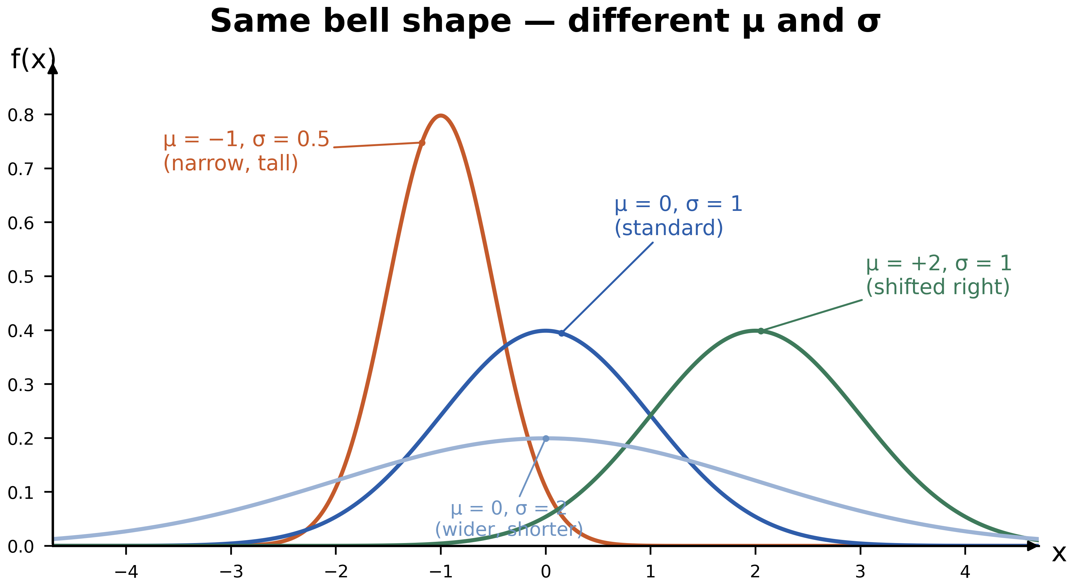
• A Gaussian random variable is written $X \sim N(\mu, \sigma^2)$ where $\mu$ is the mean and $\sigma^2$ is the variance

• all Gaussian curves are bell shaped but they can be shifted (by tuning $\mu$) or stretched/squeezed (by tuning $\sigma$)

• area under all theses curves is 1

• Probability gives me a confidence/cerainity score of the belief we have on a method/result. A self driving car gets a LiDAR reading of 3.2 m to hit an obstacle, is it safe? It depends entirely on th threshold value of an acceptable uncertanity score. If $\sigma$ is less than 0.05m, then it is fine.

So what the f*ck is Singular Value Decomposition?????

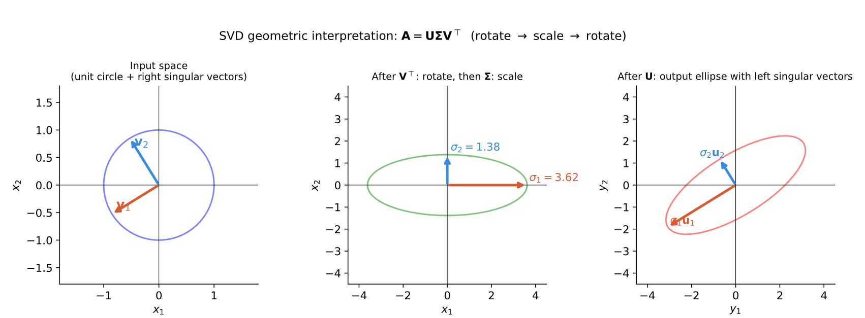
Any matrix $A$ irrespective of its shape; number of independent columns it has (rank); and the numbers present in it, can be decomposed into 3 matrices. That is it!!! It is all that is need to be known to understand SVD apart from the formula.

Now, the formula is made up of 3 matrices which basically rotate, transform, and maybe rotate any input vector again. The 3 stooges of matrices are made of the square roots of the eigen values and eigen vector of $A^TA$ and eigen vector $AA^T$.

$$A=US V^T$$

• $V$ columns are eigen vectors of $A^TA$
• $S$ is the singular values of $A$, which are the square roots of the eigen values of $A^TA$
• $U$ matrix consist of columns which are eigenvectors of $AA^T$

NOTE: SVD works only if $U$ and $V$ are orthonormal vectors. We will see why.

$$A^TA(v_{raw}) = \sigma^2(v_{raw}) \quad \textbf{--- (1)}$$ $$(A^TA-\sigma^2 I)v_{raw}=0$$ $$v_i = \frac{v_{raw}}{||v_{raw}||} \quad \textbf{--- (2)}$$

Substituting the normalised input eigen vector from eqn$\textbf{(2)}$ in eqn $\textbf{(1)}$

$$A^TA(v_{i}) = \sigma^2(v_{i}) \quad \textbf{--- (3)}$$ $$||Av_i||^2 = (Av_i)^T(Av_i) = v_i^TA^TAv_i \quad \textbf{--- (4)}$$

Substituting eqn$(3)$ in eqn$(4)$ we get

$$||Av_i||^2 = (Av_i)^T(Av_i) = v_i^TA^TAv_i = v_i^T\sigma^2(v_{i}) \quad \textbf{--- (5)}$$

Since $v_i$ is a unit vector, $v_i^Tv_i = 1$ (a scalar, not the identity matrix — that only applies when dotting a full orthonormal matrix with its transpose, e.g. $V^TV = I$). Therefore eqn$(5)$ is

$$||Av_i|| = \sigma \quad \textbf{--- (6)}$$

we know that the magnitude of $Av_i$ from eqn$(6)$

In eqn$(3)$ multiply both sides by $A$

$$AA^TA(v_{i}) = \sigma^2(Av_{i}) \quad \textbf{--- (7)}$$

normalising $Av_i$ we get

$$u_i=\frac{Av_i}{\sigma_i} \quad \textbf{--- (8)}$$

If we stack this relationship horizontally for all $n$ vector dimensions simultaneously, it maps perfectly to an equivalent matrix-matrix multiplication:

$$A \underbrace{\begin{bmatrix} \mathbf{v}_1 & \mathbf{v}_2 & \cdots & \mathbf{v}_n \end{bmatrix}}_{V} = \underbrace{\begin{bmatrix} \mathbf{u}_1 & \mathbf{u}_2 & \cdots & \mathbf{u}_m \end{bmatrix}}_{U} \underbrace{\begin{bmatrix} \sigma_1 & & \\ & \sigma_2 & \\ & & \ddots \end{bmatrix}}_{\Sigma}$$

This simplifies neatly down to:

$$AV = U\Sigma$$

Because $V$ is an orthogonal matrix built from an orthonormal basis of eigenvectors, its inverse is identical to its transpose ($V^{-1} = V^\top$). Right-multiplying both sides by $V^\top$ completely isolates $A$:

$$AVV^\top = U\Sigma V^\top$$ $$A = U\Sigma V^\top$$

So we have answered why we are using orthonormal eigenvectors and values of $A^TA$ for decomposing the matrix $A$ with the above derivation.

$Singular \: Value \: Decomposition$

Why did you even bring up mahalanobis distance and singular value decomposition together?

Look at the formulas of Mahalanobis distance and SVD they look similar. But that isn’t enough, we need to answer if Mahalanobis distance is doing SVD. This intuition is partly right. Mahalanobis distance is prefere because the formula converts an anisotropic distribution (uneven) to isotropic distribution.

From the previous formulas we can infer that covariance matrix is

$$\Sigma_{cov} = \frac{1}{n-1}\mathbf{X_c^T}\mathbf{X_c}$$ $$\mathbf{X_c} = US V^T$$

Substituting:

$$\mathbf{X_c^T X_c} = (USV^\top)^\top(USV^\top) = VS^\top U^\top USV^\top = VS^2V^\top$$

(using $U^\top U = I$ and $S^\top S = S^2$ since $S$ is diagonal)

Therefore:

$$\Sigma_{cov} = \frac{1}{n-1}\mathbf{V S^2 V^\top}$$

Note the order — it’s $VS^2V^\top$, not $V^\top S^2 V$. This matters: it tells you $V$ (not $V^\top$) holds the eigenvectors as its columns, matching the standard eigendecomposition convention $\Sigma = V\Lambda V^\top$.

Hence eigenvalues of $\Sigma_{cov}$

$$\lambda_i = \frac{\sigma^2_i}{n-1}$$

where $\sigma_i$ are the singular values of $\mathbf{X_c}$.

---

Is Mahalanobis distance doing SVD?

Short answer: partly right, partly wrong. Mahalanobis distance uses the same underlying machinery as SVD — rotation by eigenvectors, scaling by eigenvalues — but it is not performing SVD itself. What it’s actually doing is eigendecomposition, applied specifically to the covariance matrix, followed by a distance computation that SVD alone doesn’t give you.

What eigendecomposition actually is

For a symmetric matrix like $\Sigma$, eigendecomposition is:

$$\Sigma = V \Lambda V^\top$$

• $V$: columns are eigenvectors of $\Sigma$ (same $V$ on both sides — this only works because $\Sigma$ is symmetric)
• $\Lambda$: diagonal matrix of eigenvalues $\lambda_i$

Compare this to general SVD:

$$A = U \Sigma_A V^\top$$

• Two different matrices $U$ and $V$ — because $A$ is not necessarily symmetric, so its “natural input direction” and “natural output direction” can differ
• $\Sigma_A$ contains singular values $\sigma_i \geq 0$, not eigenvalues (which can be negative or complex for a non-symmetric $A$)

Why they coincide for $\Sigma$

Since the covariance matrix $\Sigma$ is symmetric and positive semi-definite:

• Its eigenvalues are guaranteed real and $\geq 0$
• Its eigenvectors are orthogonal
• Therefore $U = V$ in its SVD, and its singular values equal its eigenvalues exactly

So for $\Sigma$ specifically, eigendecomposition and SVD collapse into the same operation. That’s the source of the “Mahalanobis is doing SVD” intuition — it isn’t wrong, it’s just that SVD and eigendecomposition happen to be indistinguishable for this one special (symmetric PSD) case.

Building Mahalanobis distance from the eigendecomposition

Start from:

$$d_M^2 = e^\top \Sigma^{-1} e$$

Substitute $\Sigma = V\Lambda V^\top \Rightarrow \Sigma^{-1} = V\Lambda^{-1}V^\top$ (valid since $V^{-1} = V^\top$ for orthogonal $V$):

$$d_M^2 = e^\top V \Lambda^{-1} V^\top e = (V^\top e)^\top \Lambda^{-1} (V^\top e)$$

Let $\tilde{e} = V^\top e$ — this is $e$ rotated into the eigenvector basis. Then:

$$d_M^2 = \tilde{e}^\top \Lambda^{-1} \tilde{e} = \sum_{i=1}^{d} \frac{\tilde{e}_i^2}{\lambda_i} = \sum_{i=1}^{d}\left(\frac{\tilde{e}_i}{\sqrt{\lambda_i}}\right)^2 = \left\| \Lambda^{-1/2} V^\top e \right\|^2$$

The actual comparison: SVD pipeline vs Mahalanobis pipeline

Step	SVD applied to a vector ($A\mathbf{x}$)	Mahalanobis distance
1	rotate: $V^\top \mathbf{x}$	rotate: $V^\top e$
2	scale: multiply by $\sigma_i$	scale: divide by $\sqrt{\lambda_i}$
3	rotate again: $U(\cdot)$	no third rotation — take the norm instead
output	a transformed vector $\mathbf{y}$	a scalar distance $d_M$

Two concrete differences:

1. SVD stretches; Mahalanobis compresses. SVD’s $\Sigma_A$ multiplies by $\sigma_i$ (stretch). Mahalanobis’s $\Lambda^{-1/2}$ divides by $\sqrt{\lambda_i}$ (compress) — it’s undoing the natural spread of the data, not applying it.
2. SVD ends in a rotation; Mahalanobis ends in a norm. The third SVD step rotates the scaled vector back into output space, giving another vector. Mahalanobis instead takes $\|\cdot\|^2$ at that point, collapsing everything to a single number.

What this operation is actually called

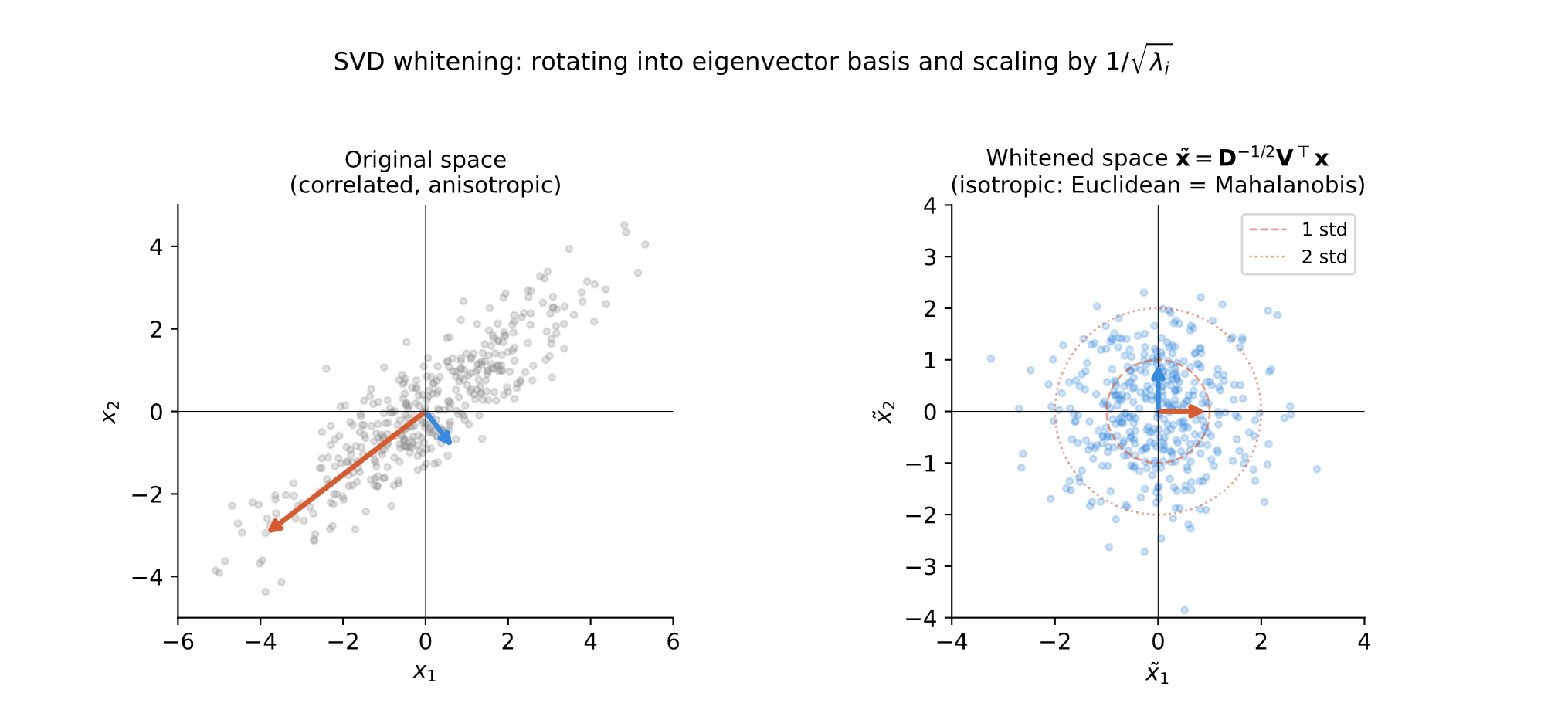
The two-step transform $\Lambda^{-1/2}V^\top$ (rotate, then scale-down) is called whitening — it takes an anisotropic (unevenly spread, correlated) distribution and turns it into an isotropic (evenly spread in all directions, uncorrelated) one:

$$\hat{e} = \Lambda^{-1/2}V^\top e \quad \Rightarrow \quad \text{Cov}(\hat{e}) = I$$

Once whitened, ordinary Euclidean distance on $\hat{e}$ is the Mahalanobis distance on $e$ — because in the whitened space every direction is equally spread, so there’s no shape left to correct for. That’s the real punchline: Mahalanobis distance = Euclidean distance, computed after first eliminating the covariance.

Verdict

Mahalanobis distance is not doing SVD. It is doing:

1. Eigendecomposition of $\Sigma$ (which happens to coincide with SVD only because $\Sigma$ is symmetric PSD)
2. A whitening transform (rotate + inverse-scale) built from that eigendecomposition
3. A final Euclidean norm — a step SVD itself never includes

The formulas look similar because both are built from the same eigenvector/eigenvalue skeleton. But SVD’s job is to decompose a general transformation into a vector output; Mahalanobis’s job is to measure a distance that accounts for the shape of the data, ending in a scalar. Same skeleton, different destinations.

References

Get a detailed understanding here →